Calculation of DGA trends - Offline vs. Online
Transformer technology redefined
Dissolved Gas Analysis (DGA) is one of the best ways to estimate transformer health, but the task of interpreting DGA results remains an active area of research. Analysing trends (or rates) is an important part of modern DGA analysis. Using trends, failures can be detected earlier, while lowering the frequency of false alarms.
But before an actual interpretation is done, the actual trend value (in ppm/day or ppm/year) has to be calculated. This is easier said than done. The IEEE Standard C57.104 gives some pointers on how to do this for offline (lab) measurements. Online (monitoring) trends are calculated differently, due to the higher frequency of available data.
This article tries to give a first overview on DGA trend calculation for both offline- and online-measurements.


Offline-DGA
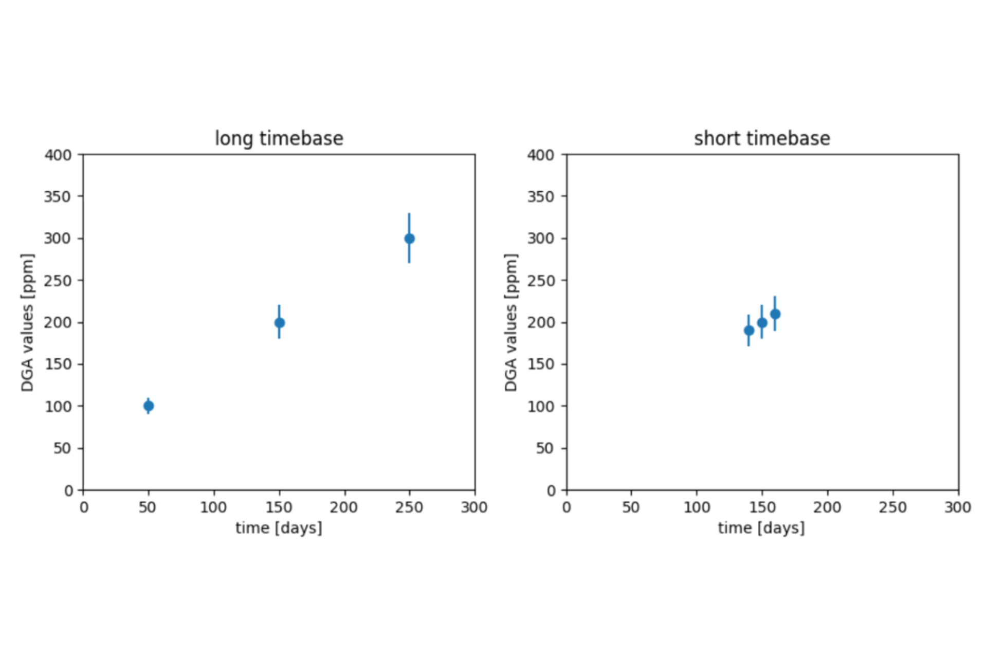
A trend can be mathematically defined as the rate of growth - difference of values divided by the difference in time. This definition would be sufficient for us if the trend is constant and if no measurement uncertainty exists. These conditions are usually not met in the context of DGA analysis. To demonstrate, let us compare two examples. In the first example (called long timebase), measurements are taken 100 days apart. In the second example (short timebase), measurements are taken 10 days apart. Both examples have a measurement uncertainty of 10%, and a true trend of 1 ppm per day. This is illustrated in the figure on the left.
Accounting for the uncertainty, it is obvious that a trend calculated from the long timebase example is more robust than the other. The uncertainty lines on the short timebase chart are even compatible with a negative trend.
Therefore, its important to keep the timebase in mind when interpreting the calculated trends. Longer timebases give more reliable trends, but this comes with a cost: If longer timebases are used, calculated trends increase slower and faults are detected later. This effect also interacts with the number of data points used to calculate a trend. If less data points are used, the uncertainty from each point has a larger influence. If more data points are used, its probable that some of the noise cancels out. More data points can be obtained by increasing the frequency of measurements or by increasing the timebase.
A trend can always be calculated by drawing a line if only two data points are available, but it's unlikely that 3 or more points will lie on a line. To calculate the trend for 3 points or more, the abovementioned standard recommends using a spreadsheet tool to calculate the "multipoint linear best fit" - another term for linear regression. If uncertainty information is available for each sample, a Bayesian linear regression analysis can be used to take this information into account.
A detection of outliers can precede the regression analysis to prevent outliers from having undue influence. A simple way to do this is to use a Hampel filter, with the disadvantage that outliers in the latest two measurements cannot be detected. Alternatively, a robust regression analysis can combine the tasks of outlier detection and trend calculation. If a Bayesian regression analysis is used, robust regression behavior can be introduced by assuming fat-tailed measurement uncertainty distributions.
Clearly, there is no single best way to do it. IEEE Standard C57.104 recommends using a simple linear regression with 3 to 6 data points, using a timebase of 4 to 24 months, using the most recent 6 data points if more are available. This results in a balance of reaction time, simplicity and accuracy that should work for many situations.
Corollary: If a transformer has yearly lab tests, the minimum of 3 data points for the timebase of 24 months will always be available directly after the latest measurement. 365 days between measurements can never be exceeded and outliers cannot happen for this schema to work.
Online-DGA
DGA monitors generate multiple data points a day. This is in stark contrast to offline measurements, where we can be lucky if multiple data points per year exist. The relative wealth of data results in quicker reaction times and better handling of outliers. Also, the automated way in which measurements are generated improves the reproducibility of the data. This is especially helpful for trend analysis.
Actually calculating this trend can still be done using a regression analysis. Usually, only the latest measurements are included in the analysis, resulting in trends that cover the last 30 days, for instance. Also, since many data points are available over that timeframe, outlier analysis can be included, reducing the influence of outliers even further.
Summarized:
This sounds like a lot of math, but luckily, we don't have to do this manually. Your DGA online monitor will do this for you.
